Introduction to CELP Coding

Do not meddle in the affairs of poles, for they are subtle and quick to leave the unit circle.

Speex is based on CELP, which stands for Code Excited Linear Prediction. This section attempts to introduce the principles behind CELP, so if you are already familiar with CELP, you can safely skip to section 8. The CELP technique is based on three ideas:

1. The use of a linear prediction (LP) model to model the vocal tract
2. The use of (adaptive and fixed) codebook entries as input (excitation) of the LP model
3. The search performed in closed-loop in a ``perceptually weighted domain''

This section describes the basic ideas behind CELP. This is still a work in progress.

Source-Filter Model of Speech Prediction

The source-filter model of speech production assumes that the vocal cords are the source of spectrally flat sound (the excitation signal), and that the vocal tract acts as a filter to spectrally shape the various sounds of speech. While still an approximation, the model is widely used in speech coding because of its simplicity.Its use is also the reason why most speech codecs (Speex included) perform badly on music signals. The different phonemes can be distinguished by their excitation (source) and spectral shape (filter). Voiced sounds (e.g. vowels) have an excitation signal that is periodic and that can be approximated by an impulse train in the time domain or by regularly-spaced harmonics in the frequency domain. On the other hand, fricatives (such as the "s", "sh" and "f" sounds) have an excitation signal that is similar to white Gaussian noise. So called voice fricatives (such as "z" and "v") have excitation signal composed of an harmonic part and a noisy part.

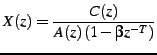
The source-filter model is usually tied with the use of Linear prediction. The CELP model is based on source-filter model, as can be seen from the CELP decoder illustrated in Figure 1.

Figure 1: The CELP model of speech synthesis (decoder)

Linear Prediction (LPC)

Linear prediction is at the base of many speech coding techniques, including CELP. The idea behind it is to predict the signal $x[n]$ using a linear combination of its past samples:

$$y[n]=\sum_{i=1}^{N}a_{i}x[n-i]$$

where $y[n]$ is the linear prediction of $x[n]$ . The prediction error is thus given by:

$$e[n]=x[n]-y[n]=x[n]-\sum_{i=1}^{N}a_{i}x[n-i]$$

The goal of the LPC analysis is to find the best prediction coefficients $a_{i}$ which minimize the quadratic error function:

$$E=\sum_{n=0}^{L-1}\left[e[n]\right]^{2}=\sum_{n=0}^{L-1}\left[x[n]-\sum_{i=1}^{N}a_{i}x[n-i]\right]^{2}$$

That can be done by making all derivatives $\frac{\partial E}{\partial a_{i}}$ equal to zero:

$$\frac{\partial E}{\partial a_{i}}=\frac{\partial}{\partial a_{i}}\sum_{n=0}^{L-1}\left[x[n]-\sum_{i=1}^{N}a_{i}x[n-i]\right]^{2}=0$$

For an order $N$ filter, the filter coefficients $a_{i}$ are found by solving the system $N\times N$ linear system $\mathbf{Ra}=\mathbf{r}$ , where

$$\mathbf{R}=\left[\begin{array}{cccc} R(0) & R(1) & \cdots & R(N-1... ...& \vdots & \ddots & \vdots\\ R(N-1) & R(N-2) & \cdots & R(0)\end{array}\right]$$

$$\mathbf{r}=\left[\begin{array}{c} R(1)\\ R(2)\\ \vdots\\ R(N)\end{array}\right]$$

with $R(m)$ , the auto-correlation of the signal $x[n]$ , computed as:

$$R(m)=\sum_{i=0}^{N-1}x[i]x[i-m]$$

Because $\mathbf{R}$ is toeplitz hermitian, the Levinson-Durbin algorithm can be used, making the solution to the problem $\mathcal{O}\left(N^{2}\right)$ instead of $\mathcal{O}\left(N^{3}\right)$ . Also, it can be proven that all the roots of $A(z)$ are within the unit circle, which means that $1/A(z)$ is always stable. This is in theory; in practice because of finite precision, there are two commonly used techniques to make sure we have a stable filter. First, we multiply $R(0)$ by a number slightly above one (such as 1.0001), which is equivalent to adding noise to the signal. Also, we can apply a window to the auto-correlation, which is equivalent to filtering in the frequency domain, reducing sharp resonances.

Pitch Prediction

During voiced segments, the speech signal is periodic, so it is possible to take advantage of that property by approximating the excitation signal $e[n]$ by a gain times the past of the excitation:

$$e[n]\simeq p[n]=\beta e[n-T]$$

where $T$ is the pitch period, $\beta$ is the pitch gain. We call that long-term prediction since the excitation is predicted from $e[n-T]$ with $T\gg N$ .

Innovation Codebook

The final excitation $e[n]$ will be the sum of the pitch prediction and an innovation signal $c[n]$ taken from a fixed codebook, hence the name Code Excited Linear Prediction. The final excitation is given by:

$$e[n]=p[n]+c[n]=\beta e[n-T]+c[n]$$

The quantization of $c[n]$ is where most of the bits in a CELP codec are allocated. It represents the information that couldn't be obtained either from linear prediction or pitch prediction. In the z-domain we can represent the final signal $X(z)$ as

$$X(z)=\frac{C(z)}{A(z)\left(1-\beta z^{-T}\right)}$$

Noise Weighting

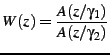
Most (if not all) modern audio codecs attempt to ``shape'' the noise so that it appears mostly in the frequency regions where the ear cannot detect it. For example, the ear is more tolerant to noise in parts of the spectrum that are louder and vice versa. In order to maximize speech quality, CELP codecs minimize the mean square of the error (noise) in the perceptually weighted domain. This means that a perceptual noise weighting filter $W(z)$ is applied to the error signal in the encoder. In most CELP codecs, $W(z)$ is a pole-zero weighting filter derived from the linear prediction coefficients (LPC), generally using bandwidth expansion. Let the spectral envelope be represented by the synthesis filter $1/A(z)$ , CELP codecs typically derive the noise weighting filter as:

$$W(z)=\frac{A(z/\gamma_{1})}{A(z/\gamma_{2})}$$ (1)

where $\gamma_{1}=0.9$ and $\gamma_{2}=0.6$ in the Speex reference implementation. If a filter $A(z)$ has (complex) poles at $p_{i}$ in the $z$ -plane, the filter $A(z/\gamma)$ will have its poles at $p'_{i}=\gamma p_{i}$ , making it a flatter version of $A(z)$ .

The weighting filter is applied to the error signal used to optimize the codebook search through analysis-by-synthesis (AbS). This results in a spectral shape of the noise that tends towards $1/W(z)$ . While the simplicity of the model has been an important reason for the success of CELP, it remains that $W(z)$ is a very rough approximation for the perceptually optimal noise weighting function. Fig. 2 illustrates the noise shaping that results from Eq. 1. Throughout this paper, we refer to $W(z)$ as the noise weighting filter and to $1/W(z)$ as the noise shaping filter (or curve).

Figure 2: Standard noise shaping in CELP. Arbitrary y-axis offset.

Analysis-by-Synthesis

One of the main principles behind CELP is called Analysis-by-Synthesis (AbS), meaning that the encoding (analysis) is performed by perceptually optimising the decoded (synthesis) signal in a closed loop. In theory, the best CELP stream would be produced by trying all possible bit combinations and selecting the one that produces the best-sounding decoded signal. This is obviously not possible in practice for two reasons: the required complexity is beyond any currently available hardware and the ``best sounding'' selection criterion implies a human listener.

In order to achieve real-time encoding using limited computing resources, the CELP optimisation is broken down into smaller, more manageable, sequential searches using the perceptual weighting function described earlier.